
Designing a Transfer Benchmark
"Can you just run it once and tell me the number?" You can. You will then spend the evening defending the number against a colleague who ran it once too and got a different one. Neither of you wrote down what you did, so the two results cannot be reconciled. The meeting ends with a decision made on whichever number was said more confidently. A benchmark that is not designed is just a transfer somebody timed.
Designing it first costs an hour. This article is that hour. It walks through the four questions a design has to answer: what to test, on what data, with what held fixed, and how many times. It leaves you with a test matrix, a way to build honest test files, and a run log template. It also gives you the one rule for summarizing results that keeps you from fooling yourself. It is part of our Benchmarking Transfer Performance series. It builds on why most transfer benchmarks lie, which cataloged the distortions this design prevents.
Start With the Question
A benchmark answers one question. Written down, the question decides everything else: which files, which protocols, which link, how many runs. Left unwritten, it drifts, and the matrix grows until nobody finishes it.
Good questions name a decision. "Will the nightly export finish inside its window if we move it from FTPS to SFTP?" leads to a decision about a migration. "Does running four uploads in parallel shorten the partner feed?" leads to a decision about a job setting. "Is the new server at least as fast as the old one for our real file mix?" leads to a decision about a cutover. Each names the job, the file mix, and the thing being varied.
Bad questions name a feeling. "How fast is the server?" has no answer, because every row of a results table is a different answer. Neither does "Is SFTP slow?", for reasons our protocol performance comparison explains. It depends on the files and the link, not on the protocol's reputation. When you catch yourself with a feeling instead of a question, ask what you would do differently depending on the result. If the answer is "nothing," there is nothing to run.
Remember: write the question at the top of the run log before the first test file is generated. Every axis of the matrix below should exist because the question needs it. An axis the question does not need is an evening you do not get back.
The Axes of the Test Matrix
A test matrix is the list of every combination you intend to measure. Each combination is a cell, and each cell gets its own set of repeated runs. Transfer benchmarks have five axes worth knowing; most questions use two or three.
File mix
The file mix is the axis that changes results the most. Per-file overhead (the fixed cost of opening, describing, and closing each file) dominates small files and vanishes for large ones. Three standard sets cover most real jobs:
- Mix A, one large file: a single file of 2 gigabytes or more. Measures the raw path: disk, network, encryption (see what changes with large files).
- Mix B, a medium batch: around 200 files of about 10 megabytes each. Measures the typical nightly export or report drop.
- Mix C, many small files: thousands of files under a few hundred kilobytes. Measures per-file overhead, which is what most "the transfer is slow" complaints are actually about. The many-small-files problem explains why.
If your real job resembles none of these, build a fourth mix that does. The next section shows how to sample the real folder.
Protocol
SFTP, FTPS, HTTPS, and, as a control on a lab LAN only, plain FTP. Each has a different per-file cost and connection pattern. Testing them fairly has its own rules, laid out in comparing protocols fairly. For the matrix, protocol is a column, not a footnote.
Concurrency
Concurrency is how many transfers run at the same time, as several files in parallel or several connections. One and four are the useful first pair; eight if the first pair shows a big gain. Parallelism helps small files and long links until the disk or the CPU saturates, and then it hurts. So this axis has a peak worth finding rather than a direction worth assuming. How the server copes with many clients at once is a separate test: load testing a transfer server.
Direction
Upload and download use different code paths on both ends and hit different disks. A server that receives quickly may serve slowly, and the reverse. If your job goes one way, test that way; if it goes both, test both, because they will not match.
Link
LAN and WAN are different experiments. The LAN test tells you what the hardware and software can do; the WAN test tells you what the job will do. Where you can, run the WAN cells from a client where the real client sits. Record the measured round-trip time. The article on latency versus bandwidth diagnosis explains why that number matters. Where you cannot, say so.
The diagram below shows the full matrix for three mixes and three protocols, and the multipliers the other axes add. It also shows the small shaded corner of it that a well-written question actually needs.
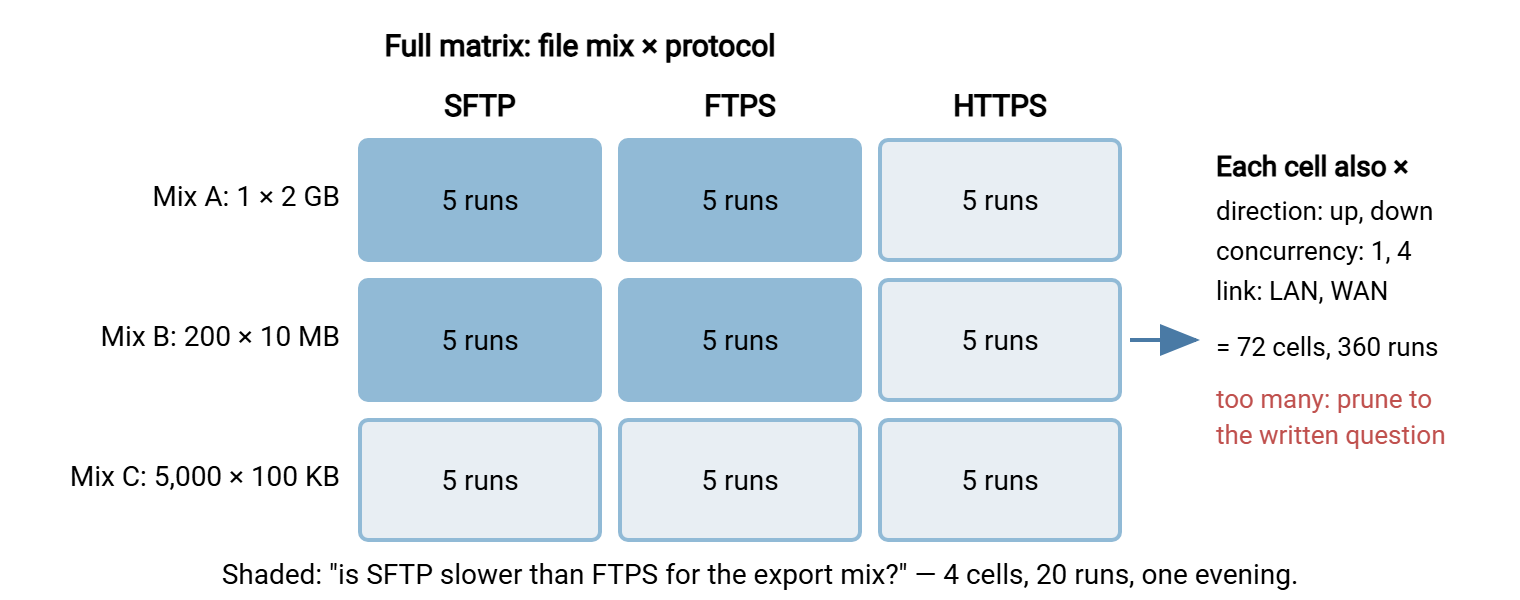
Three mixes, three protocols, two directions, two concurrency levels, and two links make 72 cells. At five runs each that is 360 runs, most of a working week at a couple of minutes per run. Nobody finishes that matrix. I have started it twice. The question is what prunes it. The export question in the diagram needs two protocols and the two mixes that resemble the export. It needs one direction, one concurrency level, and the WAN. Four cells, twenty runs, one evening. Add cells later only when a result raises a new question.
Building Honest Test Data
Test files lie in two ways: by being compressible and by being cached.
Files full of zeros compress to almost nothing. A tool that quietly compresses in flight moves a zero-filled file at a rate no real file will ever see. A protocol comparison in which one side compresses and the other does not is a comparison of nothing. Fill test files with random bytes instead. On Linux and macOS, dd reading from /dev/urandom does it in one line. On Windows, fsutil file createnew produces a zero-filled file. That is fine for sizing a disk and wrong for a benchmark. So use a short PowerShell loop that writes random blocks.
# Linux/macOS: one 2 GB file of random bytes (500 blocks of 4 MB)
dd if=/dev/urandom of=mixA_random.bin bs=4M count=500

# Linux/macOS: 5,000 small files of 100 KB each for Mix C
mkdir -p mixC && for i in $(seq 1 5000); do
  dd if=/dev/urandom of=mixC/f_$i.bin bs=100K count=1 status=none
done

# Windows PowerShell: one 2 GB file of random bytes
$rng = [System.Security.Cryptography.RandomNumberGenerator]::Create()
$buf = New-Object byte[] (4MB)
$fs  = [System.IO.File]::OpenWrite("D:\bench\mixA_random.bin")
1..500 | ForEach-Object { $rng.GetBytes($buf); $fs.Write($buf, 0, $buf.Length) }
$fs.Close()

# Freeze the set: record a checksum list so every future run uses identical files
sha256sum mixA_random.bin mixC/* > testset_checksums.txt
Caching is the second lie. The operating system keeps recently read files in memory. So a test file read twice is read from RAM the second time. If the real job reads freshly written files, that is fair; if it reads old ones, it is not. The design decision is simple. Either generate fresh files before each run, or make the large file bigger than the client's memory so it cannot be cached. Write down which you did. Cold and warm are both honest conditions. An undeclared mixture of the two is a test of the cache, published under the server's name.
The third rule is realism. If the real job is not one of the three standard mixes, sample it. List the real folder. Count how many files fall into each size band (under 100 kilobytes, under 1 megabyte, under 10, under 100, larger). Build a test set with the same proportions and roughly the same total. Ten minutes of counting beats any standard set. Freeze the set with a checksum list, as in the last line above, so a run next quarter uses the same bytes.
Controlling the Variables You Can
A benchmark compares cells. Everything that is not the axis under test should be identical between them. The list of things that quietly vary is longer than it looks.
- Same client machine, same server. Not "a similar laptop." The same hardware, the same operating system, the same client build for every cell.
- Same time window. Run all cells in one session or in the same window on consecutive nights, not some at lunch and some at midnight.
- Quiet both ends. Pause other scheduled jobs, or run in the real window and record that they were active. Know whether antivirus scans the landing folder, and keep it the same for every cell.
- Fixed tool settings. Buffer sizes, parallelism, compression, cipher: set them explicitly in the batch file or profile rather than inheriting defaults that differ between tools. Compression off for all cells unless compression is the axis under test.
- Same cache state. Fresh files or oversized files, as decided above, for every run of every cell.
- Empty destination. Clear the landing folder between runs so that overwrite behavior and directory size do not creep in.
- Outside stopwatch. Time from the shell with
timeorMeasure-Command, never from the tool's own meter. - One change at a time. If two cells differ in two ways, the result explains neither.
Bluewater Bank once broke the second bullet and nearly canceled a migration over it. Their engineer ran the FTPS cells of a statement-feed comparison at Tuesday lunchtime, then ran out of afternoon. The engineer ran the SFTP cells that night beside the backup. SFTP lost by nearly a third, and the result went into a slide. Someone in the review asked to see the run log. There was no run log. Rerun in one window, the two protocols tied.
A small harness enforces most of the list without relying on memory or on anyone's afternoon. The shape below runs one cell five times. It resets the destination and regenerates files before each run, and logs one line per run:
#!/bin/bash
# run one matrix cell five times; one CSV line per run
CELL="sftp_mixB_up_c1_wan"
for i in 1 2 3 4 5; do
  ./reset_destination.sh                 # empty the landing folder on the server
  ./make_testset.sh mixB                 # fresh random files: cold cache, same shape
  START=$(date +%s.%N)
  sftp -b batch_mixB.txt bench@xfer-test.example.net > /dev/null
  END=$(date +%s.%N)
  SECS=$(echo "$END - $START" | bc)
  echo "$CELL,$i,$(date +%H:%M),$SECS" >> runlog.csv
done
The PowerShell version is the same loop with Measure-Command around the client call and Add-Content writing the line. The language does not matter. What matters is that the reset, the regeneration, the stopwatch, and the log line happen the same way every time. No human decides whether to bother.
Recording What You Cannot Control
Some conditions cannot be held fixed. The WAN's round-trip time drifts, the server's load changes, and a switch somewhere is replaced. The only defense is to record them so a strange result can be explained later rather than argued about. The run log is that record: one line per run, with the conditions alongside the result. A CSV with the header below is enough; the fields matter more than the format.
run_id,cell,run_no,clock_time,client_host,server_host,link,rtt_ms,fileset,files,total_gb,direction,concurrency,tool_settings,cache,server_cpu_pct,other_load,wall_secs,tool_rate_mbs,notes
r0117,sftp_mixB_up_c1_wan,1,02:04,jobhost-01,xfer-test,wan,41,mixB_YYYYMMDD,200,2.0,up,1,"sftp batch; no compression; default buffers",cold,35,backup running,184.2,10.9,
r0118,sftp_mixB_up_c1_wan,2,02:08,jobhost-01,xfer-test,wan,40,mixB_YYYYMMDD,200,2.0,up,1,"sftp batch; no compression; default buffers",cold,38,backup running,181.7,11.0,
r0119,sftp_mixB_up_c1_wan,3,02:12,jobhost-01,xfer-test,wan,44,mixB_YYYYMMDD,200,2.0,up,1,"sftp batch; no compression; default buffers",cold,71,backup + AV scan,243.5,8.2,AV full scan started 02:10
A few of the fields deserve a word. rtt_ms is measured before each run with a handful of pings, because a WAN's delay is not a constant. fileset names the frozen test set, so that a future run can prove it used the same files. server_cpu_pct and other_load are read from the server during the run. The third row above shows why. That run was a third longer than its neighbors, explained by an antivirus scan that started two minutes earlier. (Scheduled for 02:10 by a different team, in a different meeting.) Without the note, that run becomes either a mystery or a quiet deletion. wall_secs is the result. tool_rate_mbs is recorded only so you can see how far the tool's meter drifts from the wall clock.
Server-side records help here, too. A server that writes per-transfer timestamps to its activity log gives you a second clock at the far end. That is how you tell "the client was slow to send" from "the server was slow to accept." Sysax Multi Server logs each session and transfer to a file or a database. Which fields a transfer log should carry is in our guide to what to log.
The Repeat-and-Summarize Rule
Every cell is run at least five times. Every cell is reported as two numbers in plain words. The median is the middle value when the five results are sorted. The spread is the fastest and slowest of the five. That is the whole statistical method, and it is enough.
The median rather than the average, because one stalled run drags an average without telling you it did. Five runs of 41, 43, 42, 58, and 42 seconds average to about 45. Their median is 42, and the 58 is visible in the spread instead of hidden in the mean. Five rather than three, because with three a single bad run is a third of your data. Five rather than ten, because ten takes twice as long and rarely changes the answer.
Two rules follow from the numbers. First, a difference smaller than the spread is not a difference. Say SFTP's median is 182 seconds with a spread of 178 to 190. FTPS's median is 176 with a spread of 171 to 188. The spreads overlap, and the honest verdict is "no meaningful difference for this mix." Second, a wide spread is a finding in itself. If the five runs of one cell range from 180 to 250 seconds, something uncontrolled is in play (a competing job, a flapping link, a scan). The right move is to find it in the run log and rerun, not to compare a noisy median against a clean one.
| Cell | Five runs (seconds) | Median | Spread | Verdict |
|---|---|---|---|---|
| SFTP, mix B, up, WAN | 184, 182, 178, 190, 181 | 182 | 178 to 190 | Clean |
| FTPS, mix B, up, WAN | 176, 171, 188, 174, 179 | 176 | 171 to 188 | Clean; overlaps SFTP — a tie |
| SFTP, mix C, up, WAN | 742, 758, 981, 749, 760 | 758 | 742 to 981 | One outlier; check the log, rerun |
Present every cell this way and resist the urge to compute percentages from single runs. "SFTP was 3 percent slower" sounds precise. "SFTP and FTPS tied for the export mix, both about three minutes" is what the data actually says. It survives a skeptical reader. How to lay the whole thing out on one page is covered in reporting results and catching regressions.
Rule of thumb: five runs, median and spread, no averages, no single-run percentages. If two spreads overlap, call it a tie. If one spread is wide, find out why before you compare it with anything.
Sizing the Effort and Scheduling the Runs
Estimate the time before you commit to a matrix. The estimate is cells times five, times the expected duration of one run plus a minute for reset and regeneration. Twenty runs of three minutes is an evening. A hundred and twenty runs of ten minutes is a week of nights. A week of nights is a matrix abandoned half-done: the first cells measured carefully, the last rushed and incomparable. Prune until the total fits the time you actually have.
Runs that must happen in the real window are best scheduled rather than attended. A scheduler does not skip the reset step because it is late. A scheduled-transfer tool does this naturally. A job defined in Sysax FTP Automation runs the same transfer set on the same schedule with the same settings. Its email notification confirms each run happened. So a five-night repeat of the WAN cells needs an operator only to read the log in the morning. For scheduled jobs that survive unattended, see our guide to Task Scheduler for transfers.
Keep the harness, the test-set generator, the checksum list, and the run log together in one folder. Put the written question at the top of a short readme. That folder is the benchmark. Anyone who has it can repeat the measurement next quarter; anyone who has only the results has a number.
Designing Before Measuring
The design is short once the question exists. Pick the cells the question needs and no more. Build random, frozen, realistic test data. Hold everything else fixed and script the parts you would otherwise forget. Log the conditions you cannot fix. Run each cell five times and report median and spread in words a colleague can check. The plan fits on a page, and the page is what makes the results comparable a year later. It is also the answer to "can you just run it once and tell me the number": yes, five times, and here is what it means.
With the design in hand, one natural next step is comparing protocols fairly, which applies the matrix to the commonest question. Another is the tuning knobs worth benchmarking, which uses the same discipline to test one change at a time. For the physics behind the WAN cells, start with TCP tuning first. It covers what TCP tuning can do before any acceleration product enters the picture.
Frequently Asked Questions
How many cells should a first benchmark have?
Why do test files need random content?
Is the median really better than the average?
What if my five runs are all over the place?
Can I run the benchmark during the day to save time?
From the Sysax team: we build secure file transfer software for Windows. Sysax Multi Server is an FTP, FTPS, SFTP, and HTTPS server. Sysax FTP Automation handles scheduled, scripted transfers. Free trials are on the download page.